What is Recommender Systems (RS)?
It is a subclass of information filtering systems that are meant to predict the preferences or ratings that a user would give to a product. Recommender systems are widely used in movies, news, research articles, products, social tags, music, etc. For example, Linkedin recommends new friends to you, Amazon recommends new products, Pandora recommends musics, you name it.
There are two types of recommender systems: content-based and collaborative filtering. There are two subtypes of collaborative filtering RS: item-item and user-user.
- Content-based: If you like this item, you may also like this…
- Item-Item: Customers who likes this also likes …
- User-User: Customers who are similar to you also liked …
It is usually convenient to use Utility Matrix to show the connect between users and items.
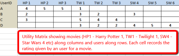
An example of Utility Matrix
Most of the time, it is sparse. The entries of it can also be 1 and 0. For example, when the item j was bought by user i, the ijth entry is 1. Often, we find a utility matrix with this kind of data shown with 0’s rather than blanks where the user has not purchased or viewed the item. However, in this case 0 is not a lower rating than 1; it is no rating at all. The goal of recommender system is to fill the blanks, find the rank top n items for each users.
Remarks:
- Since not all users like to give rate, the information we have collected were from the users who were willing to provide ratings. That is, it is biased.
- We can make inferences from users’ behavior. More generally, one can infer interest from behavior other than purchasing. For example, if an Amazon customer views information about an item, we can infer that they are interested in the item, even if they don’t buy it.
Content-based recommenders:
Features (explicit and implicit):
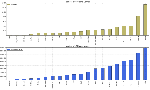
For different items, they have different features. For example, movies can use the following features: director, actors, year, genre and so on. For documents, it is common to use TF-IDF as features. Images can be characterized by tags collected from people. Features can be boolean or numerical. For example, if one feature of movies is the set of actors, then imagine that there is a component for each actor, with 1 if the actor is in the movie, and 0 if not. If one feature of movies is the average rating, then it is numerical. It is suggested to normalize the features to avoid some features are dominant.
1. User Profiles method:
User Profiles:
For content-based recommenders, we construct profiles for all users. That is,
We not only need to create vectors describing items; we need to create vectors with the same components that describe the user’s preferences from the utility matrix.
Example: Suppose items are movies, represented by boolean profiles with components corresponding to actors. Also, the utility matrix has a 1 if the user has seen the movie and is blank otherwise. If 20% of the movies that user U likes have Julia Roberts as one of the actors, then the user profile for U will have 0.2 in the component for Julia Roberts.
Example: Consider the same movie information as in Example above, but now suppose the utility matrix has nonblank entries that are ratings in the 1–5 range. Suppose user U gives an average rating of 3. There are three movies with Julia Roberts as an actor, and those movies got ratings of 3, 4, and 5. Then in the user profile of U, the component for Julia Roberts will have value that is the average of 3−3, 4−3, and 5−3, that is, a value of 1.
On the other hand, user V gives an average rating of 4, and has also rated three movies with Julia Roberts (it doesn’t matter whether or not they are the same three movies U rated). User V gives these three movies ratings of 2, 3, and 5. The user profile for V has, in the component for Julia Roberts, the average of 2−4, 3−4, and 5−4, that is, the value −2/3.
Recommending Items to Users Based on Content:
Now with the profiles of users and items, we can estimate the degree to which a user would prefer an item by computing the cosine distance between the user’s and item’s vectors.
2. Classification and Regression Algorithms:
For each user, build a classifier (for example, decision tree) or make a regression that predicts whether the user will like an item or not, or predicts the rating of all items using item profiles and utility matrices. The predictors are the features of items.
Unfortunately, classifiers of all types tend to take a long time to construct. This method is applied only when the dataset is small.
Collaborative Filtering:
Recommendation for a user U is made by looking at the users that are most similar to U in this sense, and recommending items that these users like. The process of identifying similar users and recommending what similar users like is called collaborative filtering.
How to measure similarities?
- Jaccard distance: we could ignore values in the matrix and focus only on the sets of items rated. If the utility matrix only reflected purchases, this measure would be a good one to choose. However, when utilities are more detailed ratings, the Jaccard distance loses important information.
- Cosine distance: when treat blanks as zeros, it is questionable. Since 0 represents dislike.
- Rounding the data: for example, treat ratings 1 and 2 as 0; 3, 4, and 5 as 1. Then use cosine distance.
- Normalize rates: subtract user’s average rating before using cosine distance.
The Duality of Similarity
The distances used in finding similar users can be used to find similar items. But there are two ways the symmetry is broken in practice.
- To make recommendation for user 1, we can firstly find similar users to user 1 and then get ratings from the (weighted by similarity) average rating of similar users. However, it is not symmetric for items.
- The similarity of items makes more sense than that of users.
User-User collaborative filtering:
Let 


where 
Since some users may rate higher and some tend to rate lower, take this fact into consideration, then we can also predict 


Item-Item collaborative filtering:
Similar to user-user collaborative filtering, we can use the average rating of similar items to item i as the rating by user x to item i: i.e. 
Generally, the item-item collaborative filtering performs better then the user-user approach, since items are simpler than users. But user-user approach can be done once, while item-item approach can’t.
Complexity:
The expensive step is finding k most similar users or items, and the complexity is O(|U|), where |U| is the size of the utility matrix.
One can use KNN, dimensional reduction or cluster algorithms, such as hierarchical clustering to find similar users or items.
Cluster:
For example, if there are N items, then make N/2 clusters. Use the average as the rating of user i to cluster j. After that, cluster M users to be M/2 clusters. And so on. To predict the rating of user x to item j, just find which clusters they belong to and use the average rating as the prediction.
Dimensional Reduction: UV decomposition
Suppose the utility matrix is m by n (m users and n items). Then we can decompose it to be two matrices: M~UV, U (m by d) and V (d by n). U characterizes users and V characterizes items. Here ~ means UV approximates M at non-blank entries. How to measure the closeness? We use RMSE(root -mean – square – error): 

How to get U and V so that RMSE is minimized?
- Preprocessing of the utility matrix M: subtract the average rate from user i
, then $m^*_{ij}-\bar{m^*_j}$. The order of the normalizing can be changed, though the result may be different. The third option is
. When make prediction, don’t forget to undo the normalization.
- Initialize U and V. One can choose matrices with equal elements, so that the element of UV equals the average of all non-blank elements of M. Or you can make a protuberance to that by a small number
and
follows uniform distribution or a normal distribution. But such initialization can not guarantee that the global optimal will be obtained, so you may initialized U and V many times.
- Then update the elements of U and V. For example, we are go update
to
, x be chosen so that RMSE is minimized among all options of x. (Taking derivative and set it to be 0.) What order should we follow when update the elements of U and V? You can do it row-by-row, or make a permutation of the list 1,2,3,…,N (N is the number of all elements to be updated), then follow that order. One element can be visited more than once.
- When to stop? Set a threshold, when the improvement of RMSE is less than the threshold, we stop. Or the improvement of RMSE for individual elements are too little, we stop on that element.
Gradient descent or Stochastic Gradient descent can be used. One problem is overfitting. To avoid that, one can do the procedure above many times and average the results U and V.
Pros and Cons of Collaborative filtering:
Pros: It works for any kind o items (no feature selection needed.)
Cons:
- Need enough users.
- Utility matrix is sparse.
- Hard to find users that have rated the same items.
- It becomes hard for ‘first’ user or ‘first’ item.
- Popularity bias: tends to recommend popular items.
Solutions:
- Hybrid methods
- Combine two or more recommenders. Global baseline and collaborative filtering.
Some remarks:
- Users are multi-facetted, so Top k recommendations may be very redundant. We may consider diverse recommendations.
- Interests change over time.


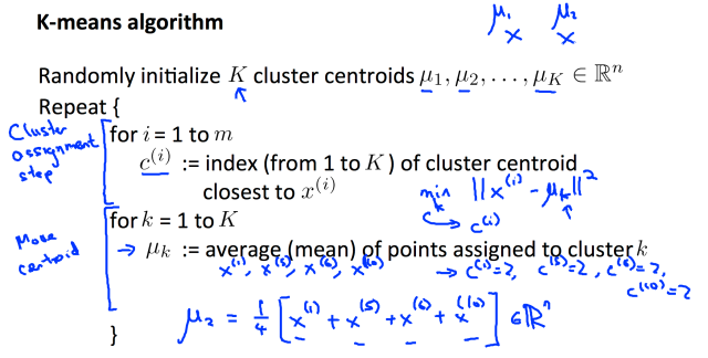

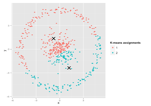
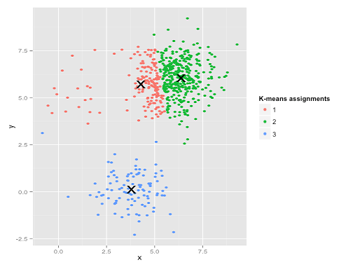
 is encoded by its nearest center and (2) each center must be at the centroid of points it owns. The algorithm will terminate in a state at which neither (1) or (2) change the configuration. The reason is as follows: there are only a finite number of ways of partitioning m records into K groups. So there are only a finite number of possible configurations in which all centers are the centroids of the points they own. If the configuration changes on an iteration, it must have improved the cost function. So each time the configuration changes it must go to a configuration it is never been to before. So if it tried to go on forever, it would eventually run out of configurations.
 , and σ → 0.
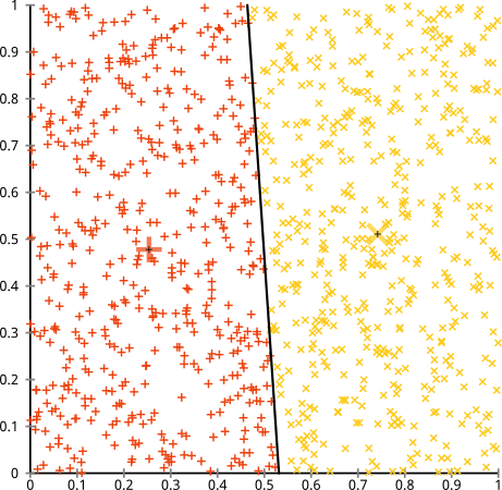
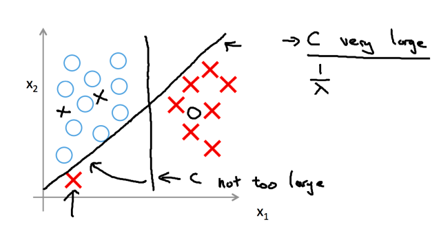
 . To separate the two classes using a hyperplane (a line in the simplified case), one reasonable choice as the best hyperplane is the one that represents the largest separation, or margin, between the two classes. In Figure 1, the red line is the best.
 , where
  . The larger
  is (
is ( ), the more confident we are to predict that
  ; the smaller
  ), the more confident we are to predict that
  . If we choose
  as the decision boundary, then the far a point is away from the decision boundary, the more confident we are about the prediction. But for the points near the boundary, a slight change of the parameters
  may lead to different predictions. So it would be nice if we can find a decision boundary such that the distances of all training points to the boundary are greater than some threshold. That’s the idea of margin.
 and
and  .
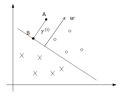
. . For a training example, the functional margin is defined to be
  . By the distance formula, it is easy to see that
 is the distance from
  , the functional margin is the same as the geometric margin. For a training set, the functional margin and the geometric margin are defined to be the minimum functional and geometric margin over all margins of the samples in the training set:
 and
and  .
.
 . This point is important in the following optimazition problem.
 s.t.
s.t. 
 s.t.
s.t. (*)
(*) s.t.
s.t. (**)
(**)
 is convex if Q is positive semidefinite. Since its Hessian matrix is Q.
 ; when
  the lost function is
  .
.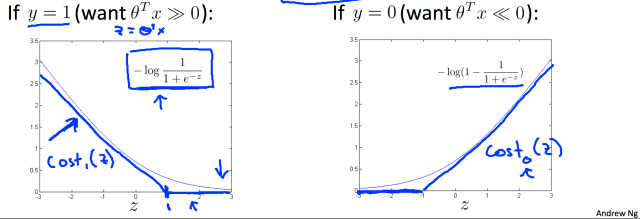
 and
and  as above, which are approximations to the lost function in logistic regression.
 , the lost function of SVM is
 .
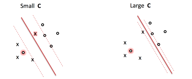
. not just larger than 0; if
  not just less than 0.
 subject to
  if
if  if
if 
 is a vector. In the polynomial case, for example,
  . If
. If  then predict 1; otherwise, predict 0. The elements of
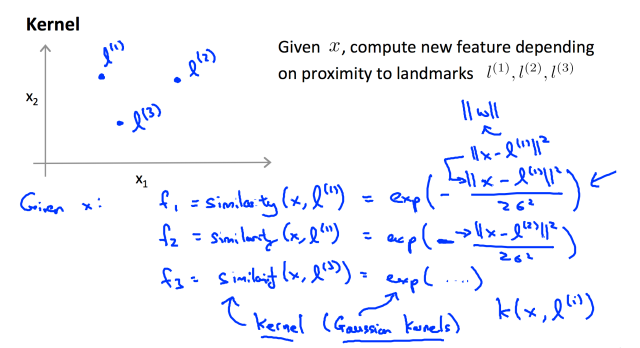
![f_i\in[0,1]](https://s0.wp.com/latex.php?latex=f_i%5Cin%5B0%2C1%5D&bg=ffffff&fg=333333&s=0&c=20201002) . The more similar, the more closer to 1.
. The more similar, the more closer to 1. . And
. And  . Then the cost function becomes
 .
. is the logistic function.
 and so on, then logistic model is not the best choice. Probably you should consider Neural networks.
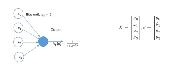
 , which are the predictors. The output is
  . The elements of
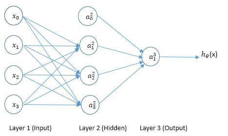
 is the ith unit(neuron) in the
  th layer.
  is the matrix of weights from layer l to layer
  .
.


 with
with  .
. and
and 
} = x}")

} = \Theta^{(l)} a^{(l)}}")
} = g(z^{(l+1)})}")

 = a^{(L)}}")
 units and the
  th layer has
  units, then the size of the weights matrix
  is
is 

 ), we expect
  be a vector with length K. If
 ![h_{\theta}(x)=e_i=[0,0,\cdots,1,\cdots, 0]^T](https://s0.wp.com/latex.php?latex=h_%7B%5Ctheta%7D%28x%29%3De_i%3D%5B0%2C0%2C%5Ccdots%2C1%2C%5Ccdots%2C+0%5D%5ET&bg=ffffff&fg=333333&s=0&c=20201002) , the sample is identified to be the ith class.
, the sample is identified to be the ith class. are m samples. We rewrite
  if the label of the ith sample is in the sth class.
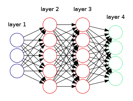

![\displaystyle \begin{array}{rcl} J(\Theta) & = & -\frac{1}{m} \bigg[\sum _{i=1}^m \sum_{k=1}^K y_k^{(i)} \log h_{\theta}(x^{(i)})_k + (1-y_k^{(i)})\log(1 - h_{\theta}(x^{(i)})_k) \bigg] \\ & + & \frac{\lambda}{2m} \sum_{l=1}^{L-1} \sum _{i=1}^{s_l} \sum _{j=1}^{s_{l+1}}(\Theta _{ji}^{(l)})^2, \end{array}](https://s0.wp.com/latex.php?latex=%5Cdisplaystyle+%5Cbegin%7Barray%7D%7Brcl%7D+J%28%5CTheta%29+%26+%3D+%26+-%5Cfrac%7B1%7D%7Bm%7D+%5Cbigg%5B%5Csum+_%7Bi%3D1%7D%5Em+%5Csum_%7Bk%3D1%7D%5EK+y_k%5E%7B%28i%29%7D+%5Clog+h_%7B%5Ctheta%7D%28x%5E%7B%28i%29%7D%29_k+%2B+%281-y_k%5E%7B%28i%29%7D%29%5Clog%281+-+h_%7B%5Ctheta%7D%28x%5E%7B%28i%29%7D%29_k%29+%5Cbigg%5D+%5C%5C+%26+%2B+%26+%5Cfrac%7B%5Clambda%7D%7B2m%7D+%5Csum_%7Bl%3D1%7D%5E%7BL-1%7D+%5Csum+_%7Bi%3D1%7D%5E%7Bs_l%7D+%5Csum+_%7Bj%3D1%7D%5E%7Bs_%7Bl%2B1%7D%7D%28%5CTheta+_%7Bji%7D%5E%7B%28l%29%7D%29%5E2%2C+%5Cend%7Barray%7D+&bg=ffffff&fg=000000&s=0 "\displaystyle \begin{array}{rcl} J(\Theta) & = & -\frac{1}{m} \bigg[\sum _{i=1}^m \sum_{k=1}^K y_k^{(i)} \log h_{\theta}(x^{(i)})_k + (1-y_k^{(i)})\log(1 - h_{\theta}(x^{(i)})_k) \bigg] \\ & + & \frac{\lambda}{2m} \sum_{l=1}^{L-1} \sum _{i=1}^{s_l} \sum _{j=1}^{s_{l+1}}(\Theta _{ji}^{(l)})^2, \end{array}")
 at the jth unit in the lth layer.
} = a^{(L)} - y}")

} = (\Theta^{(l)})^T \delta^{(l + 1)} .* g'(z^{(l)})}")

 . The “error” is related to the partial derivatives in this way:
}}J(\Theta) = \delta^{(l+1)}(a^{(l)})^T + \lambda \Theta}") .
.} = 0,\text{ for }l = 1, ..., L-1}")

} = x^{(i)}}")
}\text{ for }l=2,...,L\text{ using forward propagation (Algorithm 1)}}")
}, \text{compute } \delta^{(l)} \text{ for } l = L, ..., 2\text{ using the backpropagation algorithm (Algorithm 2)}}")
} = \Delta^{(l)} + \delta^{(l+1)}(a^{(l)})^T \text{ for }l=L-1, ..., 1}")


 times the number of input units. If more than one hidden layer, use the same number of hidden units in every layer. The more hidden units the better, the constrain here is the burden in computational time that increases with the number of hidden units.
 . Randomly initialize the parameters
 ![{\theta_{ij} \in [-\epsilon, \epsilon]}](https://s0.wp.com/latex.php?latex=%7B%5Ctheta_%7Bij%7D+%5Cin+%5B-%5Cepsilon%2C+%5Cepsilon%5D%7D&bg=ffffff&fg=000000&s=0 "{\theta_{ij} \in [-\epsilon, \epsilon]}") . Initializing
. Initializing  for all
  will result in problems. Basically all hidden units will have the same value, which is clearly undesirable.