Exploratory Analysis of Movielen Dataset using Python

The MovieLens 20M dataset:

GroupLens Research has collected and made available rating data sets from the MovieLens web site (http://movielens.org). The data sets were collected over various periods of time, depending on the size of the set.  20 million ratings and 465,564 tag applications applied to 27,278 movies by 138,493 users. Includes tag genome data with 12 million relevance scores across 1,100 tags. Released 4/2015; updated 10/2016 to update links.csv and add tag genome data. The download address is https://grouplens.org/datasets/movielens/20m/. The size is 190MB. More details can be found here:http://files.grouplens.org/datasets/movielens/ml-20m-README.html

There are 6 tables:

1. ratings.csv (userId, movieId, rating,timestamp)
2. movies.csv (movie, title, genres)
3. tags.csv (userId, movieId, tag, timestamp)
4. links.csv (movieId, imdbId, tmdbId)
5. genome_score.csv (movieId, tagId, relevance)
6. genome_tag.csv (tag, tagId)

 

Import packages and load datasets:

import pandas as pd
import numpy as np
import matplotlib.pyplot as plt
import re
import seaborn as sns

movies_pd=pd.read_csv('movies.csv')
rates_pd =pd.read_csv('ratings.csv')
links_pd=pd.read_csv('links.csv')
tags_pd=pd.read_csv('tags.csv')
genome_scores_pd=pd.read_csv('genome-scores.csv')
genome_tags_pd=pd.read_csv('genome-tags.csv')

rates_pd.head()

This is how rates_pd looks like.

	userId	movieId	rating	timestamp
0	1	2	3.5	1112486027
1	1	29	3.5	1112484676
2	1	32	3.5	1112484819
3	1	47	3.5	1112484727
4	1	50	3.5	1112484580

We convert timestamp to normal date form and only extract years.

import datetime
def convert_time(timestamp):
    date=datetime.datetime.fromtimestamp(
    int(timestamp)).strftime('%Y-%m-%d %H:%M:%S')
    return int(date[0:4])
rates_pd['year']=rates_pd['timestamp'].apply(convert_time)

Next, we calculate the average rating over all movies in each year.

avg_rates_year=rates_pd[['year','rating']].groupby('year').mean()

 

This is the head of the movies_pd dataset.

	movieId	title	genres
0	1	Toy Story (1995)	Adventure|Animation|Children|Comedy|Fantasy
1	2	Jumanji (1995)	Adventure|Children|Fantasy
2	3	Grumpier Old Men (1995)	Comedy|Romance
3	4	Waiting to Exhale (1995)	Comedy|Drama|Romance
4	5	Father of the Bride Part II (1995)	Comedy

We extract the publication years of all movies.

def year(title):
    year=re.search(r'\(\d{4}\)', title)
    if year:
       year=year.group()
       return int(year[1:5])
    else:
    return 0
movies_pd['year']=movies_pd['title'].apply(year)

Since there are some titles in movies_pd don’t have year, the years we extracted in the way above are not valid. We set year to be 0 for those movies.

sub=movies_pd[movies_pd['year']!=0]

fig1, (ax3,ax4) = plt.subplots(2,1,figsize=(20,12))
plt.subplot(211)
plt.plot(sub.groupby(['year']).count()['title_new'])
plt.title('Number of movies vs Years',fontsize=16)

plt.subplot(212)
a2=plt.plot(avg_rates_year)
plt.title('Average ratings vs genres',fontsize=16)
plt.grid(True)
plt.tight_layout()
fig.savefig('Number of Movies and average ratings VS years.jpg')

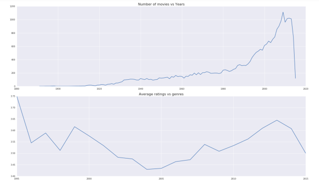
The picture shows that there is a great increment of the movies after 2009. But the average ratings over all movies in each year vary not that much, just from 3.40 to 3.75.

Next we extract all genres for all movies. That is, for a given genre, we would like to know which movies belong to it.

First, we split the genres for all movies.

import re
def genres_str(x):
    if x=='(no genres listed)':
        keys=['no_genres']
    else:
        keys= re.sub('[|]', ' ', x)
        keys=keys.split()
return keys
movies_pd['genres_split']=movies_pd['genres'].apply(genres_str)

all_genres=['Action','Adventure','Animation',"Children",
 "Comedy","Crime","Documentary","Drama",
 "Fantasy",'Film-Noir','Horror','Musical',
 'Mystery','Romance','Sci-Fi','Thriller',
 'War','Western','IMAX','no_genres']
#genres_classify[genre] gives the moviesIds which can be classified to be genre.
values=[]
for i in range(len(all_genres)):
    values.append([])
genres_classify=dict(zip(all_genres, values))

for i in range(movies_pd.shape[0]):
     for genre in movies_pd.loc[i,'genres_split']:
         genres_classify[genre].append(movies_pd.loc[i,'movieId'])

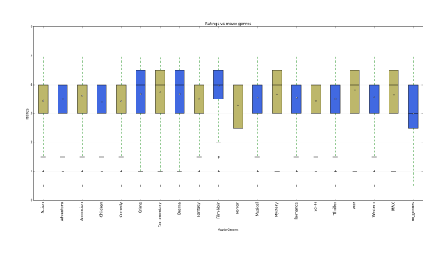
Now we can consider the  distributions of the ratings for each genre.

data=[]
for g in all_genres:
    #sub is all ratings for the movies in the genres g.
    sub=np.array(rates_pd[rates_pd['movieId'].isin(genres_classify[g])].rating)
    data.append(sub)

from matplotlib.patches import Polygon
#boxplot the ratings vs genres
fig, ax1 = plt.subplots(figsize=(20, 12))
fig.canvas.set_window_title('Boxplot of Movie Ratings VS Genres')
plt.subplots_adjust(left=0.075, right=0.95, top=0.9, bottom=0.25)

bp = plt.boxplot(data, notch=0, sym='+', vert=1, whis=1.5)
plt.setp(bp['boxes'], color='black')
# plt.setp(bp['whiskers'], color='black')
# plt.setp(bp['fliers'], color='red', marker='+')

# Add a horizontal grid to the plot, but make it very light in color
# so we can use it for reading data values but not be distracting
ax1.yaxis.grid(True, linestyle='-', which='major', color='lightgrey',
 alpha=0.5)

# Hide these grid behind plot objects
ax1.set_axisbelow(True)
ax1.set_title('Ratings vs movie genres')
ax1.set_xlabel('Movie Genres')
ax1.set_ylabel('ratings')

# Now fill the boxes with desired colors
boxColors = ['darkkhaki', 'royalblue']
plt.setp(bp['whiskers'], color='green')
#plt.setp(bp['fliers'], color='red', marker='+')
numBoxes=20

medians = list(range(numBoxes))
for i in range(numBoxes):
 box = bp['boxes'][i]
 boxX = []
 boxY = []
 for j in range(5):
 boxX.append(box.get_xdata()[j])
 boxY.append(box.get_ydata()[j])
 boxCoords = list(zip(boxX, boxY))
 # Alternate between Dark Khaki and Royal Blue
 k = i % 2
 boxPolygon = Polygon(boxCoords, facecolor=boxColors[k])
 ax1.add_patch(boxPolygon)
 # Now draw the median lines back over what we just filled in
 med = bp['medians'][i]
 medianX = []
 medianY = []
 for j in range(2):
 medianX.append(med.get_xdata()[j])
 medianY.append(med.get_ydata()[j])
 plt.plot(medianX, medianY, 'k')
 medians[i] = medianY[0]
 # Finally, overplot the sample averages, with horizontal alignment
 # in the center of each box
 plt.plot([np.average(med.get_xdata())], [np.average(data[i])],
 color='w', marker='*', markeredgecolor='k')

# Set the axes ranges and axes labels
ax1.set_xlim(0.5, numBoxes + 0.5)
top = 6
bottom = 0
ax1.set_ylim(bottom, top)
xtickNames = plt.setp(ax1, xticklabels=all_genres)
plt.setp(xtickNames, rotation=90, fontsize=12)
plt.savefig('genres_ratings.png')

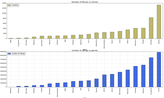
Next we make ranks by the number of movies in different genres and the number of ratings for all genres.

import operator
common={}
for g in genres_classify:
 common[g]=len(genres_classify[g])
common_sort= sorted(common.items(), key=operator.itemgetter(1))  
common_pd=pd.DataFrame(common.items(),columns=['genre', 'numbers'])
common_pd.head()

	genre	numbers
0	Mystery	1514
1	Drama	13344
2	Western	676
3	Sci-Fi	1743
4	Horror	2611

We can see that Drama is the most common genre; Comedy is the second. The most uncommon genre is Film-Noir.

Remark: Film Noir (literally ‘black film or cinema’) was coined by French film critics (first by Nino Frank in 1946) who noticed the trend of how ‘dark’, downbeat and black the looks and themes were of many American crime and detective films released in France to theaters following the war.

popular={}
i=0
for g in genres_classify:
 popular[g]=len(data[i])
 i+=1
popular_sort= sorted(popular.items(), key=operator.itemgetter(1))
popular_sort
popular_pd=pd.DataFrame(popular.items(),columns=['genre', 'number of ratings'])
popular_pd.head()
summary_genre=popular_pd.merge(common_pd,on='genre',how='inner')
summary_genre.head()

 

	genre	number of ratings
0	Mystery	5614208
1	Drama	2111403
2	Western	361
3	Sci-Fi	1669249
4	Horror	3298335

	genre	number of ratings	numbers
0	Mystery	5614208	1514
1	Drama	2111403	13344
2	Western	361	676
3	Sci-Fi	1669249	1743
4	Horror	3298335	2611
5	Film-Noir	244619	330

sort_1=summary_genre.sort_values(by='numbers')
sort_2=summary_genre.sort_values(by='number of ratings')

fig, (ax1,ax2) = plt.subplots(2,1,figsize=(20,12))

a1=sort_1.plot.bar(x='genre',y='numbers',ax=ax1,color='darkkhaki')
a1.set_title('Number of Movies vs Genres',fontsize=16)
plt.grid(True)

a2=sort_2.plot.bar(x='genre',y='number of ratings',ax=ax2,color='royalblue')
a2.set_title('number of ratings vs genres',fontsize=16)
plt.grid(True)
plt.tight_layout()

fig.savefig('Number of Movies and Number of Ratings by genres.jpg')
#plt.show()

 

Finally, we explore the users ratings for all movies and sketch the heatmap for popular movies and active users.

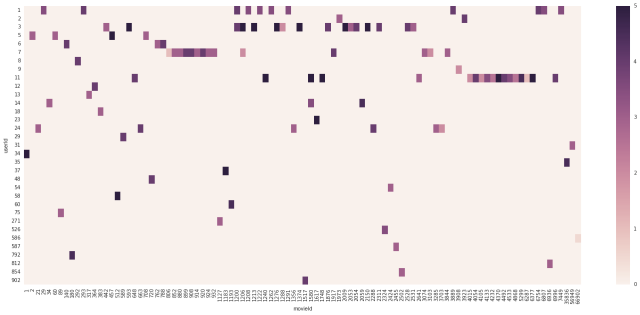
The code is below.

summary_2=rates_pd['rating'].groupby(rates_pd['userId'])
user_counts=summary_2.count().to_dict()
user_counts=pd.DataFrame(user_counts.items(), columns=['userId', 'count'])
active_users=user_counts[user_counts['count']>5000]
INDEX1=active_users.index
popular_movies=counts[counts['count']>25000]
INDEX2=popular_movies.index
INDEX=list(set(INDEX1).union(set(INDEX2)))
rates_pd_sub=rates_pd.iloc[INDEX,]
table = pd.pivot_table(rates_pd_sub, values='rating', index=['movieId'],
columns=['userId'], aggfunc=np.sum)
table_pd=pd.DataFrame(table.fillna(0))
table_pd.transpose()

#plt.figure(num=None, figsize=(20, 20))
plt.figure(num=None, figsize=(25,10), dpi=80, facecolor='w', edgecolor='k')
heatmap=sns.heatmap(table_pd.transpose())